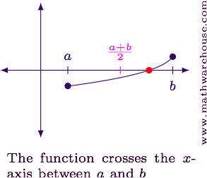
Suppose $$f(x)$$ is continuous over $$[a,b]$$, and $$f(a)$$ and $$f(b)$$ have opposite signs (see the image below). Then, the Intermediate Value Theorem tells us that the function will achieve every value between $$f(a)$$ and $$f(b)$$ at least once somewhere in $$[a,b]$$.
Since $$f(a)$$ and $$f(b)$$ have opposite signs, then we know $$0$$ is somewhere in-between. So the IVT guarantees that somewhere in $$[a,b]$$ the function will equal 0 (again, see the image below).
We approximate the location of the root by finding the midpoint of the interval at $$x = \frac{a+b} 2$$ (see image below).
Suppose $$f(x)$$ is continuous over $$[a,b]$$ and the function values at the endpoints have different signs.
Using the Bisection Method, find three approximations of the root of $$f(x) = \frac 1 4 x^2 -3$$. Determine the maximum error possible in using each approximation.
Verify the Bisection Method can be used.
We first note that the function is continuous everywhere on it's domain.
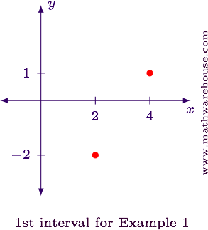
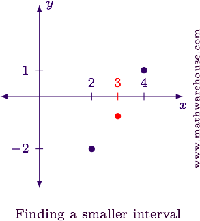
Next, we pick an interval to work with. If we pick $$x = 2$$, we see that $$f(0) = -2 < 0$$ and if we pick $$x = 4$$ we see $$f(4) = 1 >0$$. So we can start with the interval $$[2,4]$$.
Find the first approximation to the root and its associated error.
The first approximation to the root is the midpoint of our starting interval. In this case, the midpoint of $$[2,4]$$ is at $$x = 3$$.
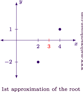
Maximum Error: Since the root has to be between $$x =2$$ and $$x = 4$$, using $$x = 3$$ as an approximation for the root means the farthest away the root could possibly be is a distance of $$\pm1$$ unit (the plus/minus is because our approximation could be too big or too small).
In general, the maximum error in using a particular approximation is half the interval length.
Use the midpoint to find a smaller interval so we can improve our approximation.
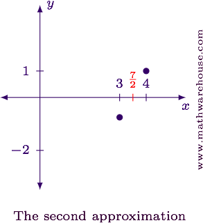
Notice that $$f(3) = \frac 1 4(3)^2 - 3 = -\frac 3 4 < 0$$. Updating our graph, we now have three points on it.
Examining this graph, we see that the root must lie between $$x=3$$ and $$x = 4$$. Consequently, this is our new interval.
Find the second approximation and its associated error.
The midpoint of the interval $$[3,4]$$ is at $$x = \frac 7 2$$. This is the second approximation.
Max Error: Our interval has a length of 1 unit, so the maximum possible error in using $$x = \frac 7 2$$ as an approximation will be $$\pm 1/2$$ of a unit.
Our graph now looks like this:
Find the next interval.
We note that $$f\left(\frac 7 2\right) = \frac 1 {16} > 0$$. Plotting this on our graph we see the following.
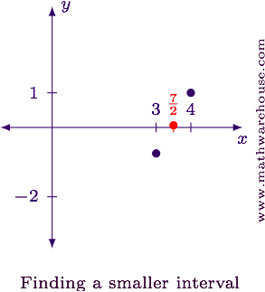
Examining this graph, we see that the root must lie between $$x = 3$$ and $$x = \frac 7 2$$. This becomes our next interval.
Find the third approximation and its associated error.
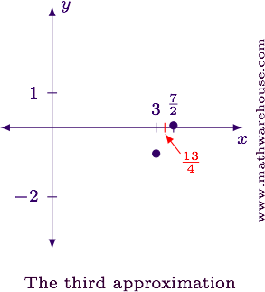
The midpoint of the interval $$\left[3, \frac 7 2\right]$$ is at $$x = \frac{13} 4$$, as shown on the graph below. This is the next approximation.
Max Error: The interval has a length of $$1/2$$, so the maximum possible error is $$\pm1/4$$ of a unit.
The table below summarizes the approximations we found and their associated errors.
$$ \begin{array}{ccc} \mbox{Approximation} & x\mbox{-value} & \mbox{Possible Error}\\ \hline 1^{st} & x = 3 & \pm1\\[6pt] 2^{nd} & x = \frac 7 2 & \pm\frac 1 2\\[6pt] 3^{rd} & x = \frac{13} 4 & \pm\frac 1 4 \end{array} $$
Use the bisection method to approximate the solution to the equation below to within less than 0.1 of its real value. Assume $$x$$ is in radians.
$$\sin x = 6 - x$$
Rewrite the equation so it is equal to 0.
$$ x - 6 + \sin x = 0 $$
The function we'll work with is $$f(x) = x - 6 + \sin x$$. Notice that the function is continuous everywhere.
Find an initial interval to work with.
Setting up a table of values, we see the following.
$$ \begin{array}{cl} x & {f(x)}\\ \hline 0 & f(0) = -6\\ 1 & f(1) \approx -4.2\\ 2 & f(2) \approx -3.1\\ 3 & f(3) \approx -2.9\\ 4 & f(4) \approx -2.8\\ 5 & f(5) \approx -2\\ 6 & f(6) \approx -0.3\\ 7 & f(7) \approx 1.7\\ \end{array} $$
The first time we see a positive function value is at $$x = 7$$. So, we can use $$[6,7]$$ as the initial interval.
Find the first approximation and its associated error.
$$ \begin{array}{ccc} \mbox{Interval} & \mbox{Midpoint} & \mbox{Max Error}\\ \hline [6, 7] & \blue{6.5} & \pm0.5 \end{array} $$
Find the 2nd interval. Use this new interval to determine the 2nd approximation. The first line of the table is included for completeness. The new work is on the second line.
$$ \begin{array}{cccc|cc} {\mbox{Finding the New Interval}}&&&& \mbox{Next Approximation}\\[6pt] f(\mbox{left}) & f(\mbox{mid}) & f(\mbox{right}) & \mbox{New Interval} & \mbox{Midpoint} & \mbox{Max Error}\\ \hline &&{\mbox{Starting Interval:}}& [6,7] & 6.5 & \pm0.5\\ f(\red 6)\approx-0.28 & f(\red{6.5})\approx 0.72 & f(7)\approx 1.66 & [6, 6.5] & \blue{6.25} & \pm0.25 \end{array} $$
Repeat Step 4 until the associated error is less than 0.1 units.
$$ {\mbox{Finding the 3rd Approximation}} \\ \\ \begin{array}{cccc|cc} &&{\mbox{Finding the New Interval}}&&&{\mbox{Next Approximation}} \\[8pt] f(\mbox{left}) & f(\mbox{mid}) & f(\mbox{right}) & \mbox{New Interval} & \mbox{Midpoint} & \mbox{Max Error}\\ \hline &&{\mbox{Starting Interval:}}& [6,7] & 6.5 & \pm0.5\\ f(6)\approx-0.28 & f(6.5)\approx 0.72 & f(7)\approx 1.66 & [6, 6.5] & 6.25 & \pm0.25\\ f(\red 6)\approx-0.28 & f(\red{6.25})\approx 0.22 & f(6.5)\approx 0.72 & [6,6.25] & \blue{6.125} & \pm0.125 \end{array} $$
$$ {\mbox{Finding the 4th Approximation}}\\[6pt] \\ \\ \begin{array}{cccc|cc} &&{\mbox{Finding the New Interval}}&&&{\mbox{Next Approximation}} \\[8pt] f(\mbox{left}) & f(\mbox{mid}) & f(\mbox{right}) & \mbox{New Interval} & \mbox{Midpoint} & \mbox{Max Error}\\ \hline &&{\mbox{Starting Interval:}}& [6,7] & 6.5 & \pm0.5\\ f(6)\approx-0.28 & f(6.5)\approx 0.72 & f(7)\approx 1.66 & [6, 6.5] & 6.25 & \pm0.25\\ f(6)\approx-0.28 & f(6.25)\approx 0.22 & f(6.5)\approx 0.72 & [6,6.25] & 6.125 & \pm0.125\\ f(6) \approx-0.28 & f(\red{6.125})\approx-0.03 & f(\red{6.25})\approx 0.22 & [6.125,6.25] & \blue{6.1875} & \pm0.0625 \end{array} $$
The solution to the equation is approximately $$6.1875$$. This approximation is accurate to within $$\pm 0.0625$$ units.
Find the third approximation from the bisection method to approximate the value of $$\sqrt[3] 2$$.
Find (make) a non-linear function with a root at $$\sqrt[3] 2$$.
We are interested in knowing the approximate value of $$x = \sqrt[3] 2$$. We use this equation to build a non-linear function with a root at the appropriate value.
$$ \\ \begin{align*} x & = \sqrt[3] 2\\ x^3 & = 2\\ x^3 - 2 & = 0 \end{align*} \\ $$
We'll use the function $$f(x) = x^3 - 2$$. Notice that the function is continuous everywhere.
Setup and work through the table as in the previous example. The approximations are in blue. The new intervals are in red.
$$ \begin{array}{cccc|cc} &&{\mbox{Finding the New Interval}}&&{\mbox{Next Approximation}} \\[8pt] f(\mbox{left}) & f(\mbox{mid}) & f(\mbox{right}) & \mbox{New Interval} & \mbox{Midpoint} & \mbox{Max Error}\\ \hline &&{\mbox{Starting Interval:}}& [0,2] & \blue 1 & \pm 1\\ f(0)=-2 & f(\red 1) = -1 & f(\red 2) = 6 & [1, 2] & \blue{1.5} & \pm0.5\\ f(\red 1) = -1 & f(\red{1.5})\approx 1.4 & f(2)=6 & [1,1.5] & \blue{1.25} & \pm0.25 \end{array} $$
$$\sqrt[3] 2 \approx \blue{1.25}$$ with a possible error of $$\pm 0.25$$. (Even with only 3 approximations, we're pretty close! The calculator tells us $$\sqrt[3] 2 \approx 1.25992$$
We know the first approximation is within $$0.5(b-a)$$ of the actual value of the root. Similarly,
In general, the $$n^{th}$$ approximation will be within $$0.5^n(b-a)$$ of the actual value. This allows us to determine ahead of time how many iterations are needed to achieve a desired degree of accuracy, as in the following example.
The function $$f(x) = x^4 - 5$$ has a positive root that is less than 3. If we started the bisection method with the interval $$[0,3]$$, how many iterations would it take before our approximation is within $$10^{-4}$$ of the actual value?
Solve $$0.5^n(b-a)=0.01$$ for $$n$$ when $$a = 0$$ and $$b = 3$$
$$ \\ \begin{align*} 0.5^n(3 -0) & = 10^{-4}\\ 0.5^n(3) & = 10^{-4}\\ 0.5^n & = \frac{10^{-4}} 3\\[6pt] n\ln(0.5) & = \ln\left(\frac 1 {30000}\right)\\[6pt] -n\ln 2 & = -\ln(30000)\\[6pt] n & = \frac{\ln 30000}{\ln 2}\\[6pt] & \approx 14.87 \end{align*} \\ $$
We would need at least 15 iterations to ensure the accuracy desired.